Lecture 3: An Intuitive Approach to Tangents and Velocity
Today we begin to explore the key ideas of calculus. We will build our intuition by investigating two problems: the geometric problem of finding the slope of a tangent line, and the physical problem of finding the velocity of an object at a single instant in time. As we'll see, the strategy for solving both is the same.
The Tangent Problem
We all have an intuitive idea of a tangent line. For a circle, it’s a line that just "touches" the circle at one point. For a general curve, the tangent line at a point $P$ is the line that best models the curve's direction at that exact spot.
The challenge is this: to find the slope of a line, we need two points. But for the tangent line, we only know one point, $P$. So how can we find its slope? We'll use an approximation strategy. Instead of the tangent, let's start with a secant line—a line that goes through our point $P$ and a second, nearby point $Q$ on the curve. Don't worry, secant is just a fancy word meaning line that cuts through two points on a curve.
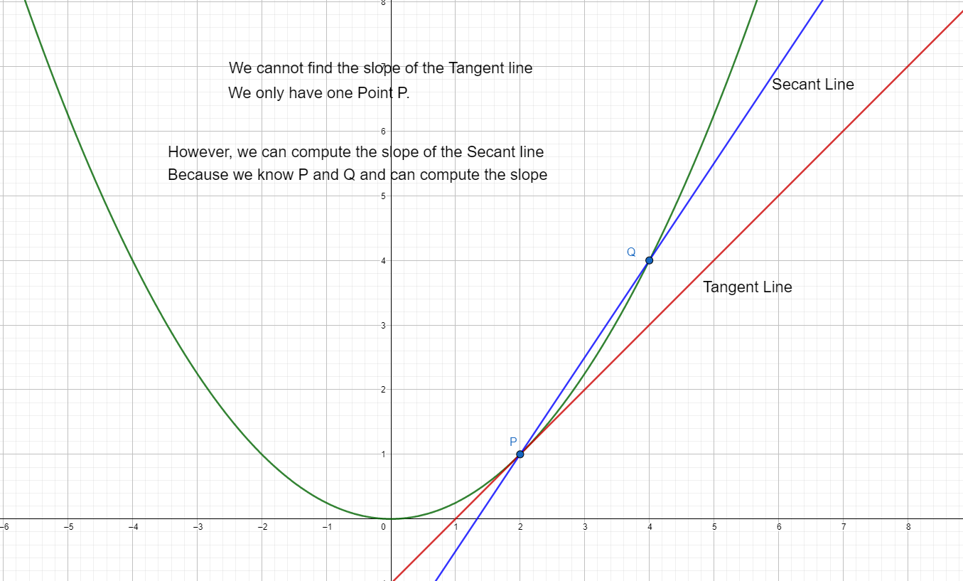
If our point $P$ has coordinates $(a, f(a))$ and our second point $Q$ has coordinates $(x, f(x))$, we can easily calculate the slope of the secant line through them:
Now the slope of the secant line is not the slope of the tangent, but it is an approximation. And we can improve this approximation by choosing our second point $Q$ to be closer and closer to $P$. As $Q$ slides along the curve towards $P$, the secant line slope changes and becomes a better and better approximation of the slope of the tangent line. The slope of the secant gets closer to the slope of the tangent.
Click here to explore how the secant line approaches the tangent line.
Example 1: Approximating a Tangent Slope
Let's estimate the slope of the tangent line to the parabola $f(x) = x^2$ at the point $P(2, 4)$.
Our point of tangency is $P(2, 4)$, so $a=2$. We will choose several points $Q(x, x^2)$ where $x$ is getting closer to 2, and we will calculate the slope of the secant line $PQ$ for each one.
The formula we'll use is $m_{sec} = \frac{x^2 - 2^2}{x - 2} = \frac{x^2 - 4}{x - 2}$.
| $x$-coordinate of Q | Point $Q$ | Slope of Secant line $PQ$, $m_{sec} = \frac{x^2-4}{x-2}$ |
|---|---|---|
| 3 | (3, 9) | $\frac{3^2 - 4}{3 - 2} = 5$ |
| 2.5 | (2.5, 6.25) | $\frac{2.5^2 - 4}{2.5 - 2} = 4.5$ |
| 2.1 | (2.1, 4.41) | $\frac{2.1^2 - 4}{2.1 - 2} = 4.1$ |
| 2.01 | (2.01, 4.0401) | $\frac{2.01^2 - 4}{2.01 - 2} = 4.01$ |
| 2.001 | (2.001, 4.004001) | $\frac{2.001^2 - 4}{2.001 - 2} = 4.001$ |
As we can see from the table, as $x$ gets closer to 2, the slope of the secant line gets closer and closer to 4. This suggests that the slope of the tangent line right at $x=2$ is approximately 4. This process of finding a value by getting closer and closer to it is the central idea of a limit.
With a slope of 4 and the point $P(2,4)$, we can compute the equation of the tangent line: $y - 4 = 4(x - 2)$, or $y = 4x - 4$.
Check Your Understanding
Problem: Consider the function $f(x) = x^3$. We want to find the slope of the tangent line at the point $P(2, 8)$. Complete the following table to estimate the slope.
| $x$-coordinate of Q | Slope of Secant line $PQ$, $m_{sec} = \frac{x^3-8}{x-2}$ |
|---|---|
| 3 | ? |
| 2.5 | ? |
| 2.1 | ? |
| 2.01 | ? |
Based on your table, what is your estimate for the slope of the tangent line at $x=2$?
The Velocity Problem
Now, let's look at a seemingly different problem from physics. Imagine you are driving a car. Your speedometer tells you your instantaneous velocity—how fast you're going at that very moment. But how could we calculate that value?
What we can easily measure is average velocity. If an object's position at time $t$ is given by a function $s(t)$, the average velocity from time $t=a$ to $t=b$ is:
This should look very familiar! It's the exact same calculation as the slope of a secant line on a position-time graph.
Just as with the tangent problem, the average velocity isn't what we ultimately want, but it's a great approximation. To estimate the instantaneous velocity at a specific moment, we can calculate the average velocity over ever decreasing intervals of time starting at that moment.
Example 2: Approximating Instantaneous Velocity
The height (in feet) of an object dropped from a tall building is given by $s(t) = 1500 - 16t^2$, where $t$ is in seconds. Let's estimate its instantaneous velocity at the moment $t=1$ second.
We will calculate the average velocity over several small time intervals that start at $t=1$. The formula is $v_{avg} = \frac{s(t) - s(1)}{t - 1}$. First, let's find the initial position at $t=1$: $s(1) = 1500 - 16(1)^2 = 1484$ ft.
| Time Interval $[1, t]$ (sec) | Average Velocity, $v_{avg} = \frac{s(t)-1484}{t-1}$ (ft/sec) |
|---|---|
| $[1, 2]$ | $\frac{s(2)-1484}{2-1} = \frac{1436-1484}{1} = -48$ |
| $[1, 1.5]$ | $\frac{s(1.5)-1484}{1.5-1} = \frac{1464-1484}{0.5} = -40$ |
| $[1, 1.1]$ | $\frac{s(1.1)-1484}{1.1-1} = \frac{1480.64-1484}{0.1} = -33.6$ |
| $[1, 1.01]$ | $\frac{s(1.01)-1484}{1.01-1} = \frac{1483.6784-1484}{0.01} = -32.16$ |
The pattern is clear. As the time interval gets smaller, the average velocity gets closer and closer to -32 ft/s. Our best estimate for the instantaneous velocity at $t=1$ second is -32 ft/sec. (The negative sign just means the object is moving downward).
Check Your Understanding
Problem: 🚗 A car's distance from home is modeled by the function $s(t) = 5t^2 + 20t$, where $s$ is in miles and $t$ is in hours. Estimate the car's instantaneous velocity (speedometer reading) at exactly $t=2$ hours by calculating the average velocity over the given intervals.
| Time Interval $[2, t]$ (hours) | Average Velocity (mph) |
|---|---|
| $[2, 3]$ | ? |
| $[2, 2.5]$ | ? |
| $[2, 2.1]$ | ? |
| $[2, 2.01]$ | ? |
Based on your table, what is your best estimate for the car's velocity at $t=2$ hours?
The insight for today is that we used the same strategy to solve two seemingly different problems. In both cases, we approximated our target value (tangent slope or instantaneous velocity) by calculating a series of approximating values (secant slopes or average velocities). By making our approximations progressively better, we could estimate the exact value. This idea of approaching a value is the concept of a limit, and it will be what we look at next.